> For the complete documentation index, see [llms.txt](https://academy.carto.com/llms.txt). Markdown versions of documentation pages are available by appending `.md` to page URLs; this page is available as [Markdown](https://academy.carto.com/advanced-spatial-analytics/spatial-analytics-for-bigquery/step-by-step-tutorials/how-to-create-a-composite-score-with-your-spatial-data.md).
# How to create a composite score with your spatial data
In this guide we show how to combine (spatial) variables into a meaningful [composite indicator](https://www.oecd.org/sdd/42495745.pdf) using CARTO Analytics Toolbox for BigQuery. Prefer a low-code approach? Check out the Workflows tutorial [Spatial Scoring: Measuring merchant attractiveness and performance](/creating-workflows/step-by-step-tutorials/spatial-scoring-measuring-merchant-attractiveness-and-performance.md).
A composite indicator is an aggregation of variables which aims to measure complex and multidimensional concepts which are difficult to define, and cannot be measured directly. Examples include [innovation](https://en.wikipedia.org/wiki/Global_Innovation_Index), [human development](https://en.wikipedia.org/wiki/Human_Development_Index), [environmental performance](https://en.wikipedia.org/wiki/Environmental_Performance_Index), and so on.
To derive a spatial score, two main functionalities are available:
* Aggregation of individual variables, scaled and weighted accordingly, into a spatial composite score ([`CREATE_SPATIAL_COMPOSITE_UNSUPERVISED`](https://docs.carto.com/data-and-analysis/analytics-toolbox-for-bigquery/sql-reference/statistics#create_spatial_composite_unsupervised))
* Computation of a spatial composite score as the residuals of a regression model which is used to detect areas of under- and over-prediction ([`CREATE_SPATIAL_COMPOSITE_SUPERVISED`](https://docs.carto.com/data-and-analysis/analytics-toolbox-for-bigquery/sql-reference/statistics#create_spatial_composite_supervised))
Additionally, a functionality to measure the internal consistency of the variables used to derive the spatial composite score is also available ([`CRONBACH_ALPHA_COEFFICIENT`](https://docs.carto.com/data-and-analysis/analytics-toolbox-for-bigquery/sql-reference/statistics#cronbach_alpha_coefficient)).
These procedures run natively on BigQuery and rely only on the resources allocated by the data warehouse.
In this guide, we show you how to use these functionalities with an example using a sample from CARTO [Spatial Features](https://carto.com/spatial-data-catalog/browser/dataset/cdb_spatial_fea_1f325a31/data) for the city of Milan (Italy) at quadbin resolution 18, which is publicly available at `` `cartobq.docs.spatial_scoring_input` ``.
As an example, we have selected as variables of interest those that better represent the target population for a wellness & beauty center mainly aimed for teenage and adult women: the female population between 15 and 44 years of age (`fempop_15_44`); the number of relevant Points of Interests (POIs), including public transportation (`public_transport`), education (`education`), other relevant pois (`pois`) which are either of interests for students (such as universities) or are linked to day-to-day activities (such as postal offices, libraries and administrative offices); and the [urbanity level](https://carto.com/blog/carto-spatial-features-urbanity-climatology-elevation) (`urbanity`). Furthermore, to account for the effect of neighboring sites, we have smoothed the data by computing the sum of the respective variables using a [k-ring](https://docs.carto.com/data-and-analysis/analytics-toolbox-for-bigquery/sql-reference/quadbin#quadbin_kring) of 20 for the population data and a k-ring of 4 for the POI data, as shown in the map below.
{% embed url="" %}
Additionally, the following map shows the average (simulated) change in annual revenue reported by all retail businesses before and after the COVID-19 pandemic. This variable will be used to identify resilient neighborhoods, i.e. neighborhoods with good outcomes despite a low target population.
{% embed url="" %}
The choice of the relevant data sources, as well as the imputation of missing data, is not covered by this set of procedures and should rely on the relevance of the indicators to the phenomenon being measured and of the relationship to each other, as defined by experts and stakeholders.
## Computing a composite score
The choice of the most appropriate scoring method depends on several factors, as shown in this diagram
First, when some measurable outcome correlated with the variables selected to describe the phenomenon of interest is available, the most appropriate choice is the supervised version of the method, available through the [`CREATE_SPATIAL_COMPOSITE_SUPERVISED`](https://docs.carto.com/data-and-analysis/analytics-toolbox-for-bigquery/sql-reference/statistics#create_spatial_composite_supervised) procedure. On the other hand, in case no such variable is available or its variability is not well captured by a regression model of the variables selected to create the composite score, the [`CREATE_SPATIAL_COMPOSITE_UNSUPERVISED`](https://docs.carto.com/data-and-analysis/analytics-toolbox-for-bigquery/sql-reference/statistics#create_spatial_composite_unsupervised) procedure should be used.
### Computing a composite score - unsupervised method
All methods included in this procedure involve a choice of a normalization function of the input variables in order to make them comparable, an aggregation function to combine them into one composite and a set of weights. As shown in the diagram above, the choice of the scoring method depends on the availability of expert knowledge: when this is available, the recommended choice for the scoring\_method parameter is `CUSTOM_WEIGHTS`, which allows the user to customize both the scaling and the aggregation functions as well as the set of weights. On the other hand, when the choice of the individual weights cannot be based on expert judgment, the weights can be derived by maximizing the variation in the data, either using a Principal Component Analysis (`FIRST_PC`) when the sample is large enough and/or the extreme values (maximum and minimum values) are not outliers or as the entropy of the proportion of each variable (`ENTROPY`). Deriving the weights such that the variability in the data is maximized means also that largest weights are assigned to individual variables that have the largest variation across different geographical units (as opposed to setting the relative importance of the individual variable as in the `CUSTOM_WEIGHTS` method): although correlations do not necessarily represent the real influence of the individual variables on the phenomenon being measured, this is a desirable property for cross-unit comparisons. By design, both the `FIRST_PC` and `ENTROPY` methods will overemphasize the contribution of highly correlated variables, and therefore, when using these methods, there may be merit in dropping variables thought to be measuring the same underlying phenomenon.
When using the `CREATE_SPATIAL_COMPOSITE_UNSUPERVISED` procedure, make sure to pass:
* The query (or a fully qualified table name) with the data used to compute the spatial composite, as well as a unique geographic id for each row
* The name of the column with the unique geographic identifier
* The prefix for the output table
* Options to customize the computation of the composite, including the scoring method, any custom weights, the custom range for the final score or the discretization method applied to the output
The output of this procedure is a table with the prefix specified in the call with two columns: the computed spatial composite score (`spatial_score`) and a column with the unique geographic identifier.
Let’s now use this procedure to compute the spatial composite score for the available different scoring methods.
#### ENTROPY
The spatial composite is computed as the weighted sum of the proportion of the [min-max scaled](https://cloud.google.com/bigquery-ml/docs/reference/standard-sql/bigqueryml-preprocessing-functions#mlmin_max_scaler) individual variables (only numerical variables are allowed), where the weights are computed to maximize the information ([entropy](https://link.springer.com/article/10.1007/s43621-021-00012-3)) of the proportion of each variable. Since this method normalizes the data using the minimum and maximum values, if these are outliers, their range will strongly influence the final output.
With this query we are creating a spatial composite score that summarizes the selected variables (`fempop_15_44`, `public_transport`, `education`, `pois`).
{% tabs %}
{% tab title="carto-un" %}
```sql
CALL `carto-un`.carto.CREATE_SPATIAL_COMPOSITE_UNSUPERVISED(
'SELECT geoid, fempop_15_44, public_transport, education, pois FROM `cartobq.docs.spatial_scoring_input`',
'geoid',
'..',
'''{
"scoring_method":"ENTROPY",
"bucketize_method":"JENKS",
"nbuckets":6
}'''
)
```
{% endtab %}
{% tab title="carto-un-eu" %}
```sql
CALL `carto-un-eu`.carto.CREATE_SPATIAL_COMPOSITE_UNSUPERVISED(
'SELECT geoid, fempop_15_44, public_transport, education, pois FROM `cartobq.docs.spatial_scoring_input`',
'geoid',
'..',
'''{
"scoring_method":"ENTROPY",
"bucketize_method":"JENKS",
"nbuckets":6
}'''
)
```
{% endtab %}
{% endtabs %}
In the options section, we have also specified the discretization method (`JENKS`) that should be applied to the output. Options for the discretization method include: `JENKS` (for natural breaks) `QUANTILES` (for quantile-based breaks) and `EQUAL_INTERVALS` (for breaks of equal width). For all the available discretization methods, it is possible to specify the number of buckets, otherwise the default option using [Freedman and Diaconis’s (1981) rule](https://robjhyndman.com/papers/sturges.pdf) is applied.
To visualize the result, we can join the output of this query with the geometries in the input table, as shown in the map below.
```sql
SELECT a.spatial_score, a.geoid, b.geom
FROM `cartobq.docs.spatial_scoring_ENTROPY_results` a
JOIN `cartobq.docs.spatial_scoring_input` b
ON a.geoid = b.geoid
```
{% embed url="" %}
#### **FIRST\_PC**
The spatial composite is computed as the first principal component score of a Principal Component Analysis (only numerical variables are allowed), i.e. as the weighted sum of the [standardized](https://cloud.google.com/bigquery-ml/docs/reference/standard-sql/bigqueryml-preprocessing-functions#mlstandard_scaler) variables weighted by the elements of the first eigenvector.
With this query we are creating a spatial composite score that summarizes the selected variables (`fempop_15_44`, `public_transport`, `education`, `pois`).
{% tabs %}
{% tab title="carto-un" %}
```sql
CALL `carto-un`.carto.CREATE_SPATIAL_COMPOSITE_UNSUPERVISED(
'SELECT geoid, fempop_15_44, public_transport, education, pois FROM `cartobq.docs.spatial_scoring_input`',
'geoid',
'..',
'''{
"scoring_method":"FIRST_PC",
"correlation_var":"fempop_15_44",
"correlation_thr":0.6,
"return_range":[0.0,1.0]
}'''
)
```
{% endtab %}
{% tab title="carto-un-eu" %}
```sql
CALL `carto-un-eu`.carto.CREATE_SPATIAL_COMPOSITE_UNSUPERVISED(
'SELECT geoid, fempop_15_44, public_transport, education, pois FROM `cartobq.docs.spatial_scoring_input`',
'geoid',
'..',
NULL,
'''{
"scoring_method":"FIRST_PC",
"correlation_thr":0.6,
"return_range":[0.0,1.0]
}'''
)
```
{% endtab %}
{% endtabs %}
In the options section, the correlation\_var parameter specifies which variable should be used to define the sign of the first principal component such that the correlation between the selected variable (`fempop_15_44`) and the computed spatial score is positive. Moreover, we can specify the (optional) minimum allowed correlation between each individual variable and the first principal component score: variables with an absolute value of the correlation coefficient lower than this threshold are not included in the computation of the composite score. Finally, by setting the `return_range` parameter we can decide the minimum and maximum values used to normalize the final output score.
Let’s now visualize the result in Builder:
{% embed url="" %}
#### **CUSTOM\_WEIGHTS**
The spatial composite is computed by first scaling each individual variable and then aggregating them according to user-defined scaling and aggregation functions and individual weights. Compared to the previous methods, this method requires expert knowledge, both for the choice of the normalization and aggregation functions (with the preferred choice depending on the theoretical framework and the available individual variables) as well as the definition of the weights.
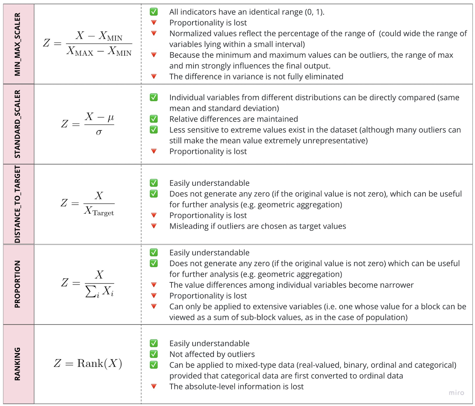
The available scaling functions are `MIN_MAX_SCLALER` (each variable is scaled into the range \[0,1] based on minimum and maximum values); `STANDARD_SCALER` (each variable is scaled by subtracting its mean and dividing by its standard deviation); `DISTANCE_TO_TARGET` (each variable’s value is divided by a target value, either the minimum, maximum or mean value); `PROPORTION` (each variable value is divided by the sum total of the all the values); and `RANKING` (the values of each variable are replaced with their percent rank). More details on the advantages and disadvantages of each scaling method are provided in the table below
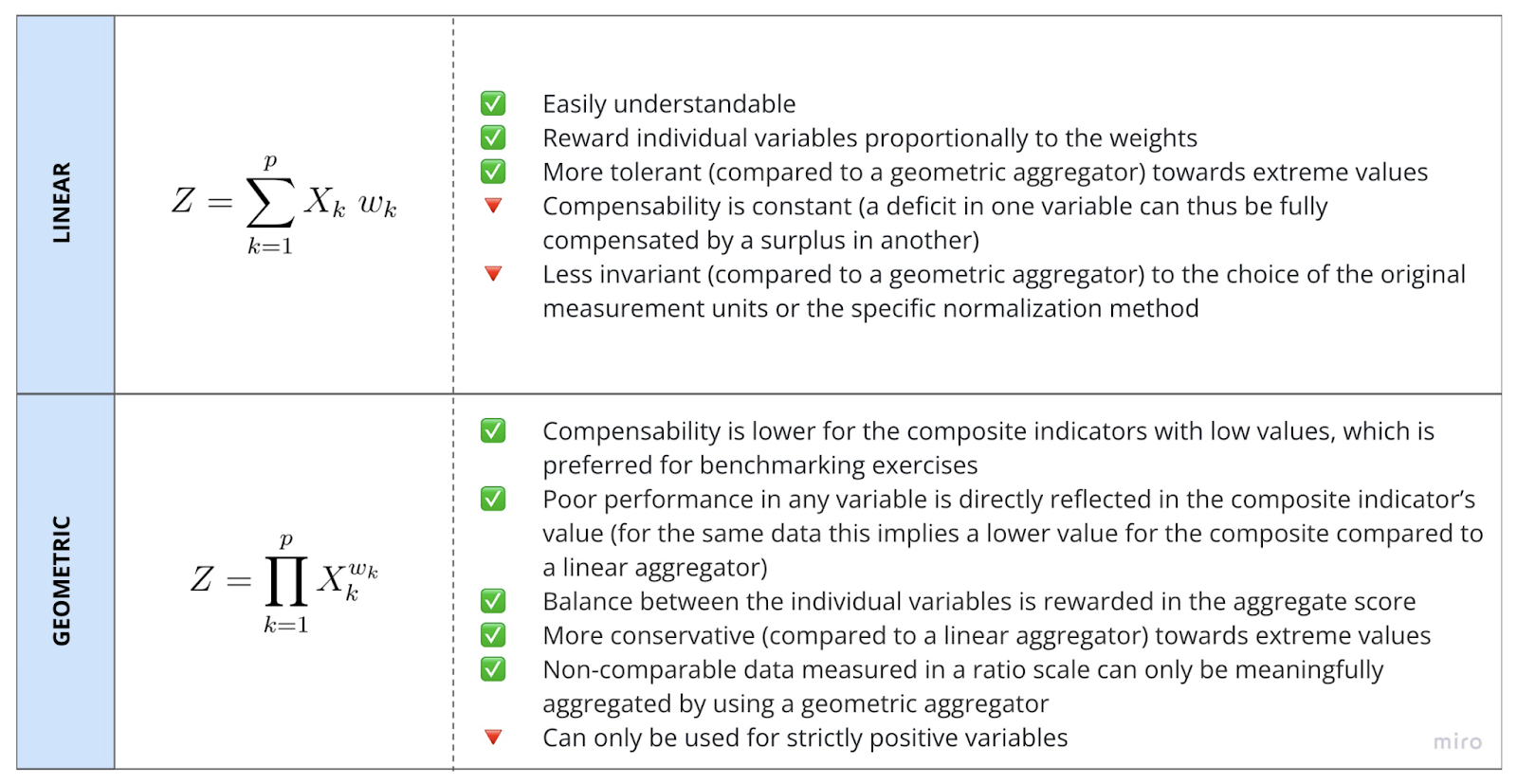
To aggregate the normalized data, two aggregation functions are available: `LINEAR` (the composite is derived as the weighted sum of the scaled individual variables multiple) and `GEOMETRIC` (the spatial composite is given by the product of the scaled individual variables, each to the power of its weight), as detailed in the following table:
In both cases, the weights express trade-offs between variables (i.e. how much an advantage on one variable can offset a disadvantage on another).
With the following query we are creating a spatial composite score by aggregating the selected variables, transformed to their percent rank, using the `LINEAR` method with the specified set of weights with sum equal or lower than 1: in this case, since we are not setting the weights for the variable `public_transport`, its weight is derived as the remainder.
{% tabs %}
{% tab title="carto-un" %}
```sql
CALL `carto-un`.carto.CREATE_SPATIAL_COMPOSITE_UNSUPERVISED(
'SELECT geoid, fempop_15_44, public_transport, education, pois, urbanity_ordinal FROM `cartobq.docs.spatial_scoring_input`',
'geoid',
'..',
'''{
"scoring_method":"CUSTOM_WEIGHTS",
"scaling":"RANKING",
"aggregation":"LINEAR",
"weights":{"fempop_15_44":0.4,"public_transport":0.2,"education":0.1,"urbanity_ordinal":0.2}
}'''
)
```
{% endtab %}
{% tab title="carto-un-eu" %}
```sql
CALL `carto-un-eu`.carto.CREATE_SPATIAL_COMPOSITE_UNSUPERVISED(
'SELECT geoid, fempop_15_44, public_transport, education, pois, urbanity_ordinal FROM `cartobq.docs.spatial_scoring_input`',
'geoid',
'..',
'''{
"scoring_method":"CUSTOM_WEIGHTS",
"scaling":"RANKING",
"aggregation":"LINEAR",
"weights":{"fempop_15_44":0.4,"public_transport":0.2,"education":0.1,"urbanity_ordinal":0.2}
}'''
)
```
{% endtab %}
{% endtabs %}
Let’s now visualize the result in Builder:
{% embed url="" %}
### Computing a composite score - supervised method
This method requires a regression model with a response variable that is relevant to the phenomenon under study and can be used to derive a composite score from the model standardized residuals, which are used to detect areas of under- and over-prediction. The response variable should be measurable and correlated with the set of variables defining the scores (i.e. the regression model should have a good-enough performance). This method can be beneficial for assessing the impact of an event over different areas as well as to separate the contribution of the individual variables to the composite by only including a subset of the individual variables in the regression model at each iteration.
When using the [`CREATE_SPATIAL_COMPOSITE_SUPERVISED`](broken://pages/S58aJqN381LZwZPKK1r4#create_spatial_composite_supervised) procedure, make sure to pass:
* The query (or a fully qualified table name) with the data used to compute the spatial composite, as well as a unique geographic id for each row
* The name of the column with the unique geographic identifier
* The prefix for the output table
* Options to customize the computation of the composite, including the [`TRANSFORM`](https://cloud.google.com/bigquery-ml/docs/bigqueryml-transform) and [`OPTIONS`](https://cloud.google.com/bigquery-ml/docs/reference/standard-sql/bigqueryml-syntax-create) clause for BigQuery [`ML CREATE MODEL` statement](https://cloud.google.com/bigquery-ml/docs/reference/standard-sql/bigqueryml-syntax-create), the minimum accepted [R2 score](https://cloud.google.com/bigquery-ml/docs/reference/standard-sql/bigqueryml-syntax-evaluate-overview), as well as the custom range or the discretization method applied to the output.
As for the unsupervised case, the output of this procedure consists in a table with two columns: the computed composite score (`spatial_score`) and a column with the unique geographic identifier.
Let’s now use this procedure to compute the spatial composite score from a regression model of the average change in annual revenue (`revenue_change`).
{% tabs %}
{% tab title="carto-un" %}
```sql
CALL `carto-un`.carto.CREATE_SPATIAL_COMPOSITE_SUPERVISED(
-- Input query
'SELECT geoid, revenue_change, fempop_15_44, public_transport, education, pois, urbanity FROM `cartobq.docs.spatial_scoring_input`',
-- Name of the geographic unique ID
'geoid',
-- Output prefix
'..',
'''{
-- BigQuery model TRANSFORM clause parameters
"model_transform":[
"revenue_change",
"fempop_15_44, public_transport, education, pois, urbanity"
],
-- BigQuery model OPTIONS clause parameters
"model_options":{
"MODEL_TYPE":"LINEAR_REG",
"INPUT_LABEL_COLS":['revenue_change'],
"DATA_SPLIT_METHOD":"no_split",
"OPTIMIZE_STRATEGY":"NORMAL_EQUATION",
"CATEGORY_ENCODING_METHOD":"ONE_HOT_ENCODING",
"ENABLE_GLOBAL_EXPLAIN":true
},
-- Additional input parameters
"r2_thr":0.4
}'''
)
```
{% endtab %}
{% tab title="carto-un-eu" %}
```sql
CALL `carto-un-eu`.carto.CREATE_SPATIAL_COMPOSITE_SUPERVISED(
-- Input query
'SELECT geoid, revenue_change, fempop_15_44, public_transport, education, pois, urbanity FROM `cartobq.docs.spatial_scoring_input`',
-- Name of the geographic unique ID
'geoid',
-- Output prefix
'..',
'''{
-- BigQuery model TRANSFORM clause parameters
"model_transform":[
"revenue_change",
"fempop_15_44, public_transport, education, pois, urbanity"
],
-- BigQuery model OPTIONS clause parameters
"model_options":{
"MODEL_TYPE":"LINEAR_REG",
"INPUT_LABEL_COLS":['revenue_change'],
"DATA_SPLIT_METHOD":"no_split",
"OPTIMIZE_STRATEGY":"NORMAL_EQUATION",
"CATEGORY_ENCODING_METHOD":"ONE_HOT_ENCODING",
"ENABLE_GLOBAL_EXPLAIN":true
},
-- Additional input parameters
"r2_thr":0.4,
"return_range":[-1.0,1.0]
}'''
)
```
{% endtab %}
{% endtabs %}
Here, the model predictors are specified in the `TRANSFORM` (`model_transform`) clause (`fempop_15_44`, `public_transport`, `education`, `pois`, `urbanity`), which can also be used to apply transformations that will be automatically applied during the prediction and evaluation phases. If not specified, all the variables included in the input query, except the response variable (`INPUT_LABEL_COLS`) and the unique geographic identifier (`geoid`), will be included in the model as predictors. In the model\_options section, we can specify all the available options for BigQuery [CREATE MODEL statement](https://cloud.google.com/bigquery-ml/docs/reference/standard-sql/bigqueryml-syntax-create) for regression model types (e.g. `LINEAR_REG`, `BOOSTED_TREE_REGRESSOR`, etc.). Another available optional parameters in this procedure is the optional minimum acceptable [R2 score](https://cloud.google.com/bigquery-ml/docs/reference/standard-sql/bigqueryml-syntax-evaluate-overview) (`r2_thr`, if the model R2 score on the training data is lower than this threshold an error is raised).
Let’s now visualize the result in Builder: areas with a higher score indicate areas where the observed revenues have increased more or decreased less than expected (i.e. predicted) and therefore can be considered resilient for the type of business that we are interested in.
{% embed url="" %}
### Computing a composite score - internal consistency
Finally, given a set of variables, we can also compute a measure of the internal consistency or reliability of the data, based on [Cronbach’s alpha coefficient](https://en.wikipedia.org/wiki/Cronbach%27s_alpha). Higher alpha (closer to 1) vs lower alpha (closer to 0) means higher vs lower consistency, with usually 0.65 being the minimum acceptable value of internal consistency. A high value of alpha essentially means that data points with high (low) values for one variable tend to be characterized by high (low) values for the others. When this coefficient is low, we might consider reversing variables (e.g. instead of considering the unemployed population, consider the employed population) to achieve a consistent direction of the input variables. We can also use this coefficient to compare how the reliability of the score might change with different input variables or to compare, given the same input variables, the score’s reliability for different areas.
The output of this procedure consists in a table with the computed coefficient, as well as the number of variables used, the mean variance and covariance.
Let’s compute for the selected variables (`fempop_15_44`, `public_transport`, `education`, `pois`) the reliability coefficient in the whole Milan’s area
{% tabs %}
{% tab title="carto-un" %}
```sql
CALL `carto-un`.carto.CRONBACH_ALPHA_COEFFICIENT(
'SELECT fempop_15_44, public_transport, education, pois FROM cartobq.docs.spatial_scoring_input',
'cartobq.docs.spatial_scoring_CRONBACH_ALPHA_results'
)
```
{% endtab %}
{% tab title="carto-un-eu" %}
```sql
CALL `carto-un-eu`.carto.CRONBACH_ALPHA_COEFFICIENT(
'SELECT fempop_15_44, public_transport, education, pois FROM cartobq.docs.spatial_scoring_input',
'cartobq.docs.spatial_scoring_CRONBACH_ALPHA_results'
)
```
{% endtab %}
{% endtabs %}
The result shows that Cronbach’s alpha coefficient in this case is 0.76, suggesting that the selected variables have relatively high internal consistency.
---
# Agent Instructions
This documentation is published with GitBook. GitBook is the documentation platform designed so that both humans and AI agents can read, navigate, and reason over technical content effectively. Learn more at gitbook.com.
## Querying This Documentation
If you need additional information that is not directly available in this page, you can query the documentation dynamically by asking a question.
Perform an HTTP GET request on the current page URL with the `ask` query parameter, and the optional `goal` query parameter:
```
GET https://academy.carto.com/advanced-spatial-analytics/spatial-analytics-for-bigquery/step-by-step-tutorials/how-to-create-a-composite-score-with-your-spatial-data.md?ask=&goal=
```
`ask` is the immediate question: it should be specific, self-contained, and written in natural language.
`goal` is optional and describes the broader end goal you are ultimately trying to accomplish on behalf of the user. GitBook uses it to tailor the answer towards what is most useful for that goal.
The response will contain a direct answer to the question and relevant excerpts and sources from the documentation.
Use this mechanism when the answer is not explicitly present in the current page, you need clarification or additional context, or you want to retrieve related documentation sections.