Featured resources

These resources have been designed to get you started. They offer an end-to-end tutorial for creating, enriching and analyzing Spatial Indexes using data freely available on the CARTO platform.

Which cell phone towers serve the most people?

Calculating traffic accident rates

Analyzing origin and destination patterns

Spatial Statistics

How Geographically Weighted Regression works

How to calculate spatial hotspots and which tools do you need?

Space-time hotspots: how to unlock a new dimension of insights

Spatial interpolation: which technique is best & how to run it

For your use case

How To Optimize Location Planning For Wind Turbines

How to use Location Intelligence to grow London's brunch scene

Optimizing Site Selection for EV Charging Stations

Using Spatial Composites for Climate Change Impact Assessment

Cloud-native telco network planning

Finding Commercial Hotspots

Analyzing 150 million taxi trips in NYC over space & time

Understanding accident hotspots

In this tutorial, we will calculate the rate of traffic accidents (number of accidents per 1,000 people) for Bristol, UK. We will be using the following datasets. The first one is available in the demo tables section of the CARTO Data Warehouse, while the latter two are freely available in our Spatial Data Catalog.

• Bristol traffic accidents (CARTO Data Warehouse)

• Census 2021 - United Kingdom (Output Area) [2021] (Office for National Statistics)

• Lower Tier Local Authority (Office for National Statistics)

Subscribing to public and premium datasetsCARTO Documentation

Step 1: Converting accident data to Spatial Indexes

In this step, you'll convert the individual accident point data to aggregated H3 cells.

1. Create a Workflow using the CARTO Data Warehouse connection.

2. First, drag the Lower Tier Local Authority data onto the canvas. It can be found under Sources > Data Observatory > Office for National Statistics.

3. Connect this to a Simple Filter component. Set the filter to do_label is equal to "Bristol, City of".

4. Next, connect the filter results to a H3 Polyfill component, and set the resolution to 9. This will create a H3 grid covering the Bristol area.

5. Now, drag the Bristol traffic accidents table onto the canvas. It can be found under Sources > Connection > CARTO Data Warehouse > demo tables.

6. Connect this to a H3 from GeoPoint component, setting the resolution of this to 9 also. This will create a H3 index for each input point.

7. Connect the output of H3 from GeoPoint to a Group by component. Set the group by column to H3, and the aggregation column to H3 (count). The result of this will be a table with a count for the number of accidents within each H3 cell.

8. In the final stage for this section, add a Join component. Connect the H3 Polyfill component to the top input, the Group by component to the bottom input, and set the join type to Left.

9. Run!

The result of this will be a H3 index covering the Bristol area with a count for the number of accidents which have taken place within each cell. Now let's put those counts into context!

Step 2: Enrich the grid with population data

In this section of the tutorial, we will enrich the H3 grid we have just created with population data from the UK Census.

1. Drag the Census 2021 - United Kingdom (Output Area) [2021] table onto the canvas from Sources > Connections > Office for National Statistics.

2. Drag an Enrich H3 Grid onto the canvas. Connect the Join component (Step 1 point 4) to the top input, and the Census data to the bottom output.

3. The component should detect the H3 and geometry columns by default. From the Variables drop down, add "ts001_001_ff424509" (total population, you can reference Variable descriptions for any dataset on our Data Observatory) and specify the aggregation method as SUM. This will estimate the total population living in each H3 cell based on the area of overlap with each Census Output Area.

Run the workflow.

Step 3: Calculating the accident rate & hotspot analysis

Now we have all of the variables collected into the H3 support geography, we can start to turn this into insights.

1. First, we'll calculate the accident rate. Connect the output of Enrich H3 Grid to a new Create Column component. Call the new column "rate".

2. Set the expression as CASE WHEN h3_count_joined IS NULL THEN 0 ELSE h3_count_joined/(ts001_001_ff424509_sum/1000) END. This code calculates the number of accidents per 1,000 people, unless there has been no accident in the area, in which case the accident rate is set to 0.

3. Now, let's explore hotspots of high accident rates . Connect the output of Create Column to a new Getis Ord component which is the hotspot function we will be using. Set the value column as "rate" (i.e. the variable we just created), the kernel to gaussian and the neighborhood size to 3. Learn more about this process here.

4. Finally, connect the results of this to a Simple Filter, and the filter condition to where the p_value is equal to or less than 0.05; this means we can be 95% confident that the locations we are looking at are a statistically significant hotspot.

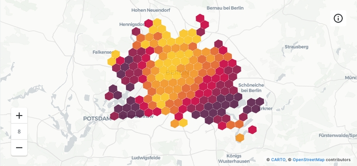
You can explore the results below!

💡 Note that to be able to visualize a H3 index in CARTO Builder, the field containing the index must be called H3.

In this tutorial, we will calculate the population living within 1km of cell towers in the District of Columbia. We will be using the following datasets, all of which can be found in the demo tables section of the CARTO Data Warehouse:

• Cell towers worldwide

• USA state boundaries

• Derived Spatial Features H3 USA

Step 1: Convert cell towers to a Spatial Index

In this step we will filter the cell towers to an area of interest (in this example, that's the District of Columbia), before converting them to a H3 index. For this, we'll follow the workflow below.

1. Create a workflow using the CARTO Data Warehouse connection and drag the three tables onto the canvas.

2. Connect the USA state boundaries table to a Simple Filter dataset, and set the filter condition for the name to equal the Colorado (or any state of your choosing!).

3. Next, connect the outcome of the Simple Filter to the bottom input (filter table) of a Spatial Filter component, and then connect the Cell towers table to the top input (source table). This should automatically detect the geometry columns in both tables. We'll keep the spatial predicate as the default "intersects"; this predicate filters the source table where any part of its geometry intersects with any part of the filter geometry.

4. Finally, connect the output of the Spatial Filter to a H3 from GeoPoint component to encode the point location as a H3 index. Ensure the resolution is the same as the Spatial Features population data; 8.

Step 2: Finding the population within 1km of each cell tower

Next, we will use K-rings to calculate the population who live roughly within 1km of each cell tower.

1. Connect the result of H3 from Geopoint to a new H3 KRing component, and set the size. You can use this documentation and this hexagon properties calculator to work out how many K-rings you need to approximate specific distances. We are working at resolution 8, where a H3 cell has a long-diagonal of approximately 1km, so we need a H3 of 1 to approximate 1km.

2. You can see in the image above that this generates a new table containing the K-rings; the kring_index is the H3 reference for the newly generated ring, which can be linked to the original, central H3 cell.

3. Next, use a Join to join the K-ring to the Spatial Features population data. Ensure the K-ring is the top input and the population data is the bottom field. Then set up the parameters so the main table column is kring_index, the secondary table column is h3 and the join type is Left.

You can see this visualized below.

Step 3: Summarizing the results

Finally, we will calculate the total population within 1km of each individual cell tower.

1. Connect the result of your last Join component to a Group by component. Set the group by column to H3 and the aggregation to population_joined with the aggregation type SUM (see above).

2. You should now know the total population for each H3 cell which represents the cell towers. The final step is to join these results back to the cell tower data so we can identify individual towers. To do this, add a final Join component, connecting H3 from GeoPoint (created in Step 1, point 4) to its top input, and the result of Group by to the bottom input. The columns for both main and secondary table should be H3, and you will want to use a Left join type to ensure all cell tower records are retained.

Run!

Altogether, your workflow should look something like the example below. The final output (the second Join component) should be a table containing all of the original cell tower data, as well as a H3 index column and the population_joined_sum_joined field (you may wish to use Rename Column to rename this!).

And here are the results!